What is machine learning? What problems can machine learning solve? (case analysis)

With the advent of the era of big data, machine learning has become an important and critical tool for solving problems. Whether in industry or academia, machine learning is a hot topic, but academic and industrial research on machine learning has a different focus. The academic community focuses on the study of machine learning theory. The industry focuses on how to use machines. Learn to solve practical problems. Combining with the U.S. group’s practice in machine learning, we will introduce an InAcTIon series (an article with the “In Machine Learning InAcTIon series” label), introducing the basic techniques required for machine learning to solve industrial problems. Experience and skill. This article mainly combines practical problems and outlines the whole process of machine learning to solve practical problems, including key issues such as modeling problems, preparing training data, extracting features, training models, and optimizing models; several other articles will carry out these key links. Describe it in more depth.

The following are divided into 1) an overview of machine learning, 2) modeling problems, 3) preparing training data, 4) extracting features, 5) training models, 6) optimizing models, and 7) reviewing a total of 7 chapters for introduction.

Overview of machine learning: What is machine learning?

As machine learning continues to find its application in the real industry, the word has been given various meanings. The meaning of "machine learning" in this article is in line with the explanation on wikipedia, as follows: Machine learning is a scienTIfic discipline that deals with the construcTIon and study of algorithms that can learn from data.

Machine learning can be divided into unsupervised learning and supervised learning. In the industrial world, supervised learning is a more common and more valuable method. The following description is mainly introduced in this way. As shown in the following diagram, there are two processes for supervised machine learning in solving practical problems. One is the offline training process (blue arrows), which includes data screening and cleaning, feature fusing model training, and optimization models; Another process is the application process (green arrow), estimating the data that needs to be estimated, extracting features, and applying the model obtained from off-line training, and obtaining the estimated value to act on the actual product. In both processes, off-line training is the most technically challenging job (a lot of work on the online estimation process can reuse the work of off-line training process), so the following describes the off-line training process.

What is a model?

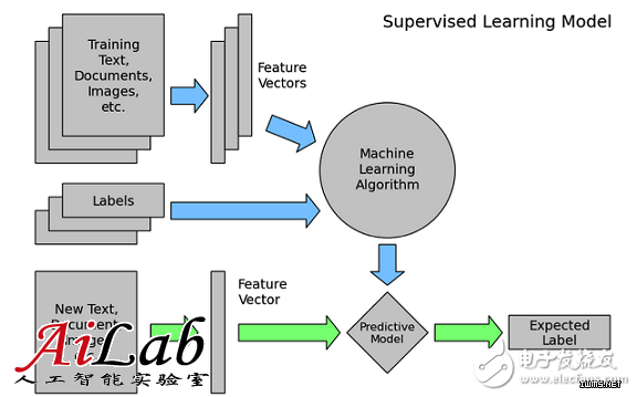
The model is an important concept in machine learning. Simply speaking, it refers to the mapping from feature space to output space; it is generally composed of the model's hypothesis function and parameter w (the following formula is an expression of the Logistic Regression model, in the training model The chapters do a little detailed explanation); The hypothesis space of a model refers to the set of all output spaces corresponding to a given model. The commonly used models in the industry include Logistic Regression (abbreviated as LR), Gradient Boosting Decision Tree (abbreviated GBDT), Support Vector Machine (abbreviated as SVM), and Deep Neural Network (abbreviated as DNN).

Model training is based on training data, obtaining a set of parameters w, making the specific target optimal, that is to obtain the optimal mapping from the feature space to the output space, how to achieve specific, see the training model chapter.

Why use machine learning to solve problems?

At present, in the era of big data, there are data that becomes T into P everywhere, and it is difficult for simple rules to play the value of these data.

Inexpensive high-performance computing reduces the time and cost of learning based on large-scale data;

Cheap, large-scale storage enables faster and less expensive processing of large-scale data;

There are a lot of high-value issues, which make it possible to get a lot of money after spending a lot of time learning to solve problems with machine learning.

What should machine learning be used to solve?

The target problem needs great value, because machine learning has a certain price to solve the problem;

The target problem has a large amount of data available, and there is a large amount of data to make machine learning solve the problem better (as opposed to simple rules or manual);

The target problem is determined by many factors (characteristics), and the advantage of machine learning to solve the problem can be reflected (as opposed to simple rules or manual);

The goal problem needs continuous optimization because machine learning can continue to play its value based on data self-learning and iteration.

Modeling problems

This article takes DEAL (group purchase order) transaction amount estimation as an example (that is, estimating how much a given DEAL sells for a period of time) and describes how to use machine learning to solve problems. First need:

Collect information on the problem, understand the problem, and become experts on this issue;

Dismantling the problem, simplifying the problem, and converting the problem into predictable problems for the machine.

After in-depth understanding and analysis of the DEAL transaction amount, it can be decomposed into several issues as follows:

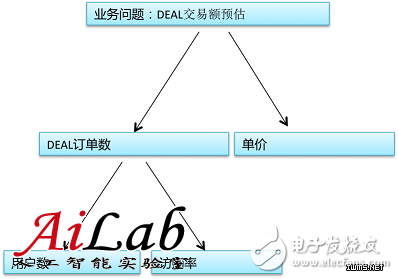A single model? Multiple models? How to choose?

After dismantling according to the above figure, there are 2 possible modes for estimating the DEAL transaction amount. One is to directly estimate the transaction amount; the other is to estimate the sub-problems, such as establishing a user number model and establishing a visit. The rate model (the number of orders that the user who visits this DEAL will purchase) will calculate the transaction amount based on the estimated value of these sub-questions.

Different methods have different advantages and disadvantages, as follows:

Mode Disadvantages Advantages Single Model 1. Estimated difficulty 2. Risk is relatively high 1. Theoretically obtain the best estimate (actually difficult) 2. Solve the problem once
Multiple models 1. Accumulation errors may occur 2. Training and application costs are high 1. Individual sub-models are easier to achieve more accurate predictions 2. Sub-models can be fused to achieve the best results

Which mode to choose?

1) If the difficulty of the problem is predictable and difficult, consider using multiple models;

2) The importance of the problem itself, the problem is very important, then consider using multiple models;

3) Multiple models can be used if they have a clear relationship and a clear relationship.

If you use multiple models, how to integrate? It can be based on the characteristics and requirements of the problem of linear fusion, or a complex fusion. Take the problem in this article as an example. There are at least two of the following:

Model selection

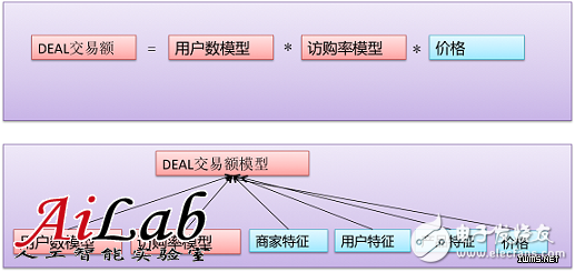
For the issue of DEAL transaction volume, we believe that direct estimation is very difficult and we hope to split into sub-problems for estimation, namely the multi-model model. In that case, it is necessary to establish a user number model and a visit rate model because machine learning solves problems in a similar manner. The following only takes the visit rate model as an example. To solve the issue of accessibility, we must first choose the model. We have the following considerations:

Main consideration

1) Select the model that is consistent with the business objectives;

2) Select the model that matches the training data and features.

There are few training data, and there are many High Level features. The “complex” nonlinear models (popular GBDT, Random Forest, etc.) are used; training data is very large, and Low Level features are more, then “simple” linear models (popular LR) are used. , Linear-SVM, etc.)

Supplementary considerations

1) Whether the current model is widely used by the industry;

2) Is there a mature open source toolkit (inside or outside the company) in the current model;

3) Whether the amount of data that the current toolkit can handle can meet the requirements;

4) Whether or not you understand the current model theory, whether you have used the model to solve the problem before.

To select the model for the actual problem, the business objective that needs to be transformed is the model evaluation objective, and the evaluation model for the conversion model is the model optimization goal; according to the different goals of the business, the appropriate model is selected. The specific relationship is as follows:

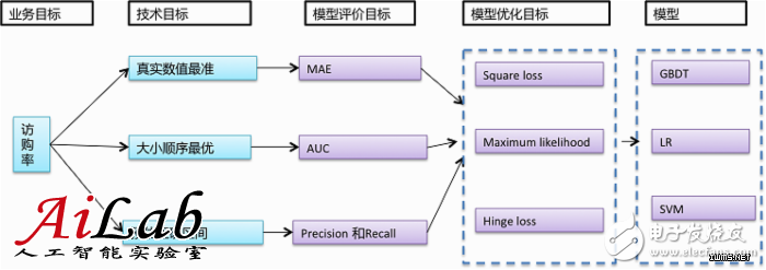
Generally speaking, it is difficult to estimate the true value (regression), size order (sequencing), and target correct range (classification) from the largest to the smallest. According to the application requirements, select the target that is as difficult as possible. For the application target of access rate estimation, we need to know at least the size order or the real value, so we can choose Area Under Curve (AUC) or Mean Absolute Error (MAE) as the evaluation target, and use Maximum likelihood as the model loss function. (Ie optimization goal). To sum up, we chose the spark version GBDT or LR, which is mainly based on the following considerations:

1) Can solve sorting or regression problems;

2) We have implemented our own algorithm, used it often, and it works well.

3) Support massive data;

4) Widely used by the industry.

Prepare training data

In-depth understanding of the problem, after selecting the appropriate model for the problem, the next step is to prepare the data; data is the root of machine learning to solve the problem. If the data is not selected correctly, the problem cannot be solved, so preparing the training data requires extra care and attention. :

be careful:

The distribution of the data to be solved is as consistent as possible;

The data distribution of the training set/test set distribution and the online prediction environment are as consistent as possible, where the distribution refers to the distribution of (x,y), not only the distribution of y;

y data noise is as small as possible, so as to eliminate y noise data;

Non-essential sampling is not required. Sampling can often cause changes in the actual data distribution. However, if the data is too large to be trained or if the positive and negative ratios are seriously out of balance (for example, over 100:1), the sampling solution is required.

Common problems and solutions

The data distribution of the problem to be solved is inconsistent:

1) The DEAL data may be very different in the access rate problem. For example, DEAL and hotel DEAL have inconsistent influence factors or performance, and need special treatment; either normalize the data in advance, or use the distribution inconsistency factor as a feature, or Train the model individually for each category of DEAL.

The data distribution has changed:

1) Train the model with data from half a year ago to predict the current data, as the data distribution may change over time and the effect may be poor. Try to use recent data training to predict the current data. Historical data can be used to reduce the weight to the model, or do transfer learning.

y data is noisy:

1) In the establishment of the CTR model, the items not seen by the user as a negative example, these items because the user did not see it was not clicked, not necessarily the user does not like not clicked, so these items are noisy . Some simple rules can be used to remove these noise negatives, such as adopting the skip-above idea, that is, the item that the user clicks on, and the Item that has not been clicked as the negative example (assuming that the user is browsing the Item from the top down).

The sampling method is biased and does not cover the entire collection:

1) In the issue of access rate, DEAL for multiple stores cannot be well estimated if only DEAL with only one store is estimated. Should guarantee the DEAL data of a store and multiple stores;

2) There is no binary classification of objective data, rules are used to obtain positive/negative cases, and rules do not cover coverage of positive/negative cases comprehensively. The data should be randomly sampled and manually annotated to ensure that the sampled data is consistent with the actual data distribution.

Training data on accessibility issues

Collect N months of DEAL data (x) and corresponding purchase rate (y);

Collecting the most recent N months, excluding holidays and other unconventional hours (keeping the distribution consistent);

Only DEAL (reduces y noise) with online duration >T and number of access users > U

Consider the DEAL sales lifecycle (keep the distribution consistent);

Consider the differences between different cities, different business districts, and different categories (keep the distribution consistent).

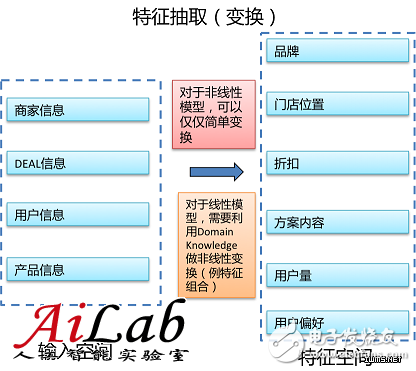
Extract features

After data filtering and cleaning are completed, the data extraction feature is required to complete the conversion from input space to feature space (see the figure below). Different feature extractions are needed for linear models or nonlinear models. Linear models require more feature extraction work and skills, while nonlinear models require relatively low feature extraction.

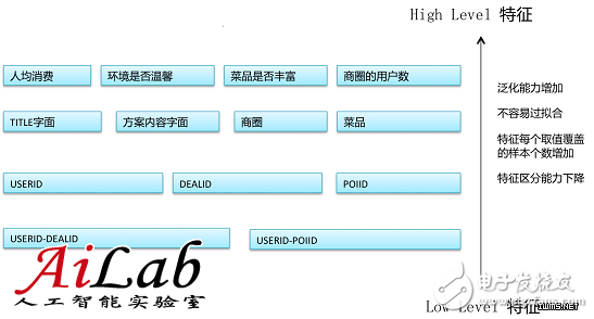
Generally, features can be classified into High Level and Low Level. High Level refers to a more generic feature, and Low Level refers to a specific feature. For example:

DEAL A1 belongs to POIA, with a per capita below 50, with a high rate of visits; DEAL A2 belongs to POIA, with a per capita above 50, and a high rate of visits; DEAL B1 belongs to POIB with a per capita below 50 and a high rate of visits; DEAL B2 belongs to POIB, with a per capita above 50 , access to the end of the rate;

Based on the above data, two characteristics can be obtained, POI (store) or per capita consumption; POI characteristics are Low Level features, and per capita consumption is a High Level feature; assuming the model learns, the following estimates are obtained:

If DEALx belongs to POIA (Low Level feature), the access rate is high; if DEALx is below 50 (High Level feature), the access rate is high.

Therefore, overall, the Low Level is relatively targeted, the coverage of a single feature is small (the data containing this feature is not much), and the number of features (dimensions) is large. The High Level is more generalized, the coverage of a single feature is larger (there are many data containing this feature), and the number of features (dimensions) is not large. The prediction of long-tailed samples is mainly influenced by the characteristics of High Level. The prediction of high frequency samples is mainly influenced by the Low Level feature.

For the issue of access rates, there are a large number of High Level or Low Level features, some of which are shown in the figure below:

Characteristics of nonlinear models

1) The High Level feature can be mainly used because the computational complexity is large, so the feature dimension should not be too high;

2) The target can be better fitted by the High Level nonlinear mapping.

Linear model features

1) The feature system should be as comprehensive as possible, both High Level and Low Level;

2) The High Level can be converted to Low Level to improve the model's fitting ability.

Feature normalization

After feature extraction, if the range of values ​​of different features varies greatly, it is better to normalize the features to achieve better results. The common normalization method is as follows:

Rescaling:

Normalize to [0,1] or [-1,1] in a similar way:

Standardization:

Set as the mean of the x distribution,

The standard deviation of the x distribution;

Scaling to unit length:

Normalized to unit length vector

Feature selection

After feature extraction and normalization, if too many features are found, which results in the model being unable to train, or it is easy to cause the model to overfit, then it is necessary to select features and select valuable features.

Filter: Assume that the feature subsets have independent effects on the model prediction. Select a feature subset and analyze the relationship between the subset and the data label. If there is some positive correlation, the feature subset is considered valid. There are many algorithms for measuring the relationship between feature subsets and data labels, such as Chi-square, Information Gain.

Wrapper: Select a feature subset to add to the original feature set, use the model for training, and compare the effects before and after the subset is added. If the effect is better, consider that the feature subset is valid, otherwise it is invalid.

Embedded: Combines feature selection with model training, such as adding L1 Norm, L2 Norm to the loss function.

Training model

After the feature extraction and processing are completed, the model training can be started. The following is a brief introduction to the simple and commonly used Logistic Regression model (hereinafter referred to as LR model) as an example.

There are m (x, y) training data, where x is the feature vector and y is the label; w is the parameter vector in the model, ie the object to be learned in the model training.

The so-called training model is to select the hypothesis function and the loss function. Based on the existing training data (x, y), continuously adjust w so that the loss function is optimal. The corresponding w is the final learning result, and the corresponding model is obtained.

Model Function 1) Hypothesis function, ie, assume there is a functional relationship between x and y:

2) Loss function, based on the above hypothesis function, constructs the model loss function (optimization goal), usually targeting the (x,y) maximum likelihood estimation in LR:

optimization

Gradient Descent

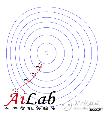
That is, w is adjusted along the direction of the negative gradient of the loss function, as shown in the figure below.

The gradient is the first derivative (see below), and there are several types of gradient drop, such as a random gradient or a batch gradient.

Stochastic Gradient Descent, randomly selecting one sample at each step

, calculate the corresponding gradient, and complete the update of w, as follows,

Batch Gradient Descent, each step calculates the gradient corresponding to all samples in the training data, w iterate along this gradient direction, ie

Newton's Method

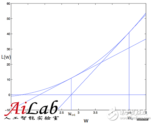
The basic idea of ​​Newton's method is to find the minimum value of L(w) by performing a second-order Taylor expansion of the objective function near the minimum point. Graphically speaking, a tangent is made at wk. The intersection of this tangent line with L(w)=0 is the next iteration point wk+1 (schematic diagram below). The updated formula for w is as follows, where the second-order partial derivative of the objective function is the famous Hessian matrix.

Quasi-Newton Methods: It is more difficult to calculate the second-order partial derivative of the objective function. The more complicated is that the Hessian matrix of the objective function can not maintain positive definite; and the Hessian matrix can be constructed without second-order partial derivatives. Inverse positive definite symmetry matrix, thus optimizing the objective function under the condition of "quasi-Newton".

BFGS: Using the BFGS formula to approximate H(w), H(w) needs to be put in memory, and O(m2) level is needed for memory;

L-BFGS: Store update matrix for a finite number of times (eg, k times)

, use these update matrices to generate new H(w), memory down to O(m) level;

OWLQN: If we introduce L1 regularization in the objective function, we need to introduce a virtual gradient to solve the problem of non-guidance of the objective function. OWLQN is used to solve this problem.

Coordinate Descent

For w, each iteration, with the other dimensions fixed, searches for only one dimension to determine the optimal descending direction (schematics are shown below). The formula is expressed as follows:

Optimization model

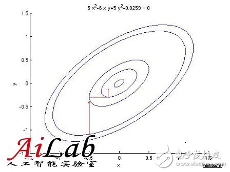
After the above-mentioned data filtering and cleaning, feature design and selection, and model training, a model is obtained, but if it is found that the effect is not good? How to do?

【First of all】

Reflect on whether the target can be estimated, and whether there are bugs in data and features.

【then】

Analyze whether the model is Overfitting or Underfitting, and optimize the data, features, and models.

Underfitting & Overfitting

Windows Tablet

Windows Tablet

C&Q Technology (Guangzhou) Co.,Ltd. , https://www.gzcqteq.com